


K-Means;with code
03 Aug 2021 | Machine Learning, Deep Learning
K-Means 실습 코드1: https://github.com/finddme/Finddme_Blog_Code/blob/master/Machine%20Learning/KMeans%EC%8B%A4%EC%8A%B51.ipynb
K-Means 실습 코드2: https://github.com/finddme/Finddme_Blog_Code/blob/master/Machine%20Learning/KMeans%EC%8B%A4%EC%8A%B52.ipynb
K-Means
-
K-Means는 클러스터링 알고리즘 중 하나이다. 클러스터링이란, 다량의 데이터를 군집화하는 기술로, 군집 간의 분산은 최대화하고 군집 내의 분산은 최소화하는 것이 목적인 알고리즘이다. K-Means알고리즘은 데이터의 영역을 대표하는 중심값(Cluster-center)을 찾아가며 데이터를 해당 Cluster에 할당하는 방식으로 작동한다.
-
데이터를 군집화하는 클러스터링과 같은 기술을은 대부분 비지도 학습 알고리즘이다. K-Means또한 비지도 학습 알고리즘에 속한다. 비지도 학습 알고리즘이란, 개발 시 정확한 작동 방향을 제시해주지 않아도 알아서 학습되는 알고리즘이다.(분류의 경우, 지도학습에 속한다)
-
K-means는 활용 분야가 매우 넓기 때문에 대표적인 데이터 마이닝 기술로 취급된다.
K-Means | 수행 과정
K-means는 EM알고리즘을 기반으로 작동된다. 즉, Expectation Step과 Maximization Step을 반복하며 학습한다. Expectation Step은 각 군집의 중심값을 찾는 단계이고, Maximization Step은 각 데이터들의 소속 클러스터를 갱신하는 단계이다. 두 단계를 수행한 후에는 중심값을 클러스터의 중앙으로 옮긴 후 다시 두 단계를 반복한다. 즉,
1. K-Means를 시작하면 중심값을 정하고, 중심에 가까운 데이터들을 해당 클러스터에 포함시킨다(EM알고리즘)
2. 중심값을 각 클러스터의 중앙으로 위치를 옮긴다.
위 두 과정을 반복하며 수행된다.
이러한 과정을 더이상 중심값의 위치가 변하지 않을 때까지 반복한다.
K-Means | 수행 준비
K-means를 수행하기 전,
1. 클러스터 개수
2. 클러스터링 수행 방식(무작위 중심값 선택, K-Means++ 등)
을 고려해 놔야 한다.
K-Means | 작동원리
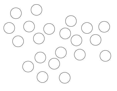
위와 같은 데이터가 있을 때, 클러스터는 3개, K-Means++ 방식으로 클러스터링을 수행해보겠다.
1. 우선 맨 처음에 랜덤으로 특정한 원소 하나를 중심값으로 설정하고, 해당 값과 가장 먼 값을 골라준다.(K-Means++방식)
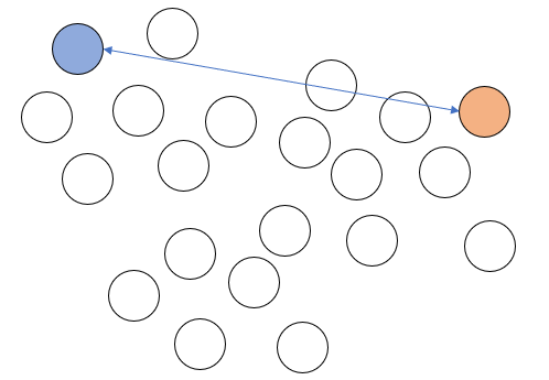
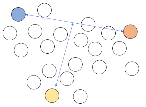
2. 그리고 두 중심값으로부터 가장 먼 원소를 또 다른 중심값으로 설정한다. 이렇게 중심값을 설정하면 세개의 중심값은 서로 가장 먼 위치에 자리하게 된다.
3. 각 데이터를 가장 가까운 중심값의 클러스터에 포함시킨다. 예를 들어 아래 그림의 회색 데이터는 1번 클러스터 중심값과 가장 가깝기 때문에 1번 클러스터에 소속된다.
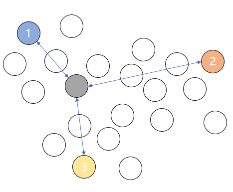
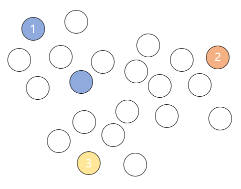
모든 데이터들에 위와 같은 과정을 수행한다.
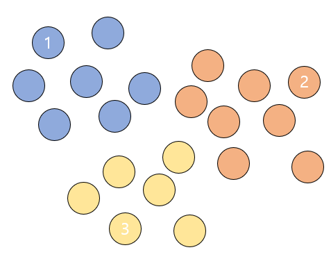
4. 군집화를 위와 같이 한 차례 마친 후에는 중심값들을 군집들의 중심으로 위치를 옮긴다.
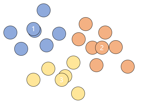
그리고 다시 모든 데이터들이 각각 어느 클러스터의 중심값과 더 가까운지 확인해주고 기존에 소속된 클러스터의 중심값보다 다른 중심값이 더 가까우면 소속 클러스터를 변경해준다.
이러한 과정을 완전한 중심값을 찾을 때 까지, 즉 중심값이 더이상 변경되지 않을 때까지 반복한다.
K-Means | 실습1
from sklearn.cluster import KMeans # KMeans 라이브러리를 불러온다.
import numpy as np
import pandas as pd
import seaborn as sns # 데이터 시각화를 위한 seaborn과 matplotlib을 불러온다.
import matplotlib.pyplot as plt
%matplotlib inline
K-Means | 실습1 | 데이터 형성
# 데이터프레임을 하나 만든다.
df1 = pd.DataFrame(columns=['x','y'], dtype = 'float')
print(df1)
Empty DataFrame
Columns: [x, y]
Index: []
# 클러스터링을 수행할 데이터를 앞서 만든 데이터프레임에 채워준다.
# 좌표평면 위에 표현할 수 있는 데이터를 넣어준다. x축, y축.
# [x값, y값]
# 총 31개.
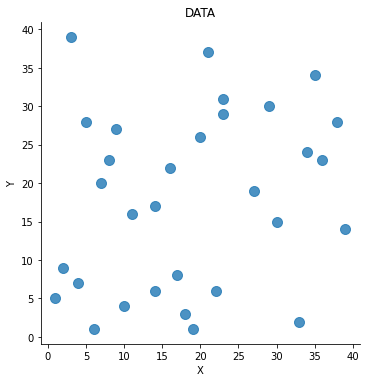
df1.loc[0] = [2, 9]
df1.loc[1] = [6, 1]
df1.loc[2] = [29, 30]
df1.loc[3] = [7, 20]
df1.loc[4] = [23, 31]
df1.loc[5] = [36, 23]
df1.loc[6] = [10, 4]
df1.loc[7] = [4, 7]
df1.loc[8] = [8, 23]
df1.loc[9] = [22, 6]
df1.loc[10] = [34, 24]
df1.loc[11] = [21, 37]
df1.loc[12] = [17, 8]
df1.loc[13] = [19, 1]
df1.loc[14] = [35, 34]
df1.loc[15] = [38, 28]
df1.loc[16] = [1, 5]
df1.loc[17] = [16, 22]
df1.loc[18] = [30, 15]
df1.loc[19] = [5, 28]
df1.loc[20] = [18, 3]
df1.loc[21] = [14, 17]
df1.loc[22] = [27, 19]
df1.loc[23] = [39, 14]
df1.loc[24] = [23, 29]
df1.loc[25] = [3, 39]
df1.loc[26] = [9, 27]
df1.loc[27] = [20, 26]
df1.loc[28] = [11, 16]
df1.loc[29] = [14, 6]
df1.loc[30] = [33, 2]
# head 함수를 사용해서 위에서 데이터를 하나하나 넣은 데이터프레임을 출력해본다.
df1.head(31)
x
y
0
2.0
9.0
1
6.0
1.0
2
29.0
30.0
3
7.0
20.0
4
23.0
31.0
5
36.0
23.0
6
10.0
4.0
7
4.0
7.0
8
8.0
23.0
9
22.0
6.0
10
34.0
24.0
11
21.0
37.0
12
17.0
8.0
13
19.0
1.0
14
35.0
34.0
15
38.0
28.0
16
1.0
5.0
17
16.0
22.0
18
30.0
15.0
19
5.0
28.0
20
18.0
3.0
21
14.0
17.0
22
27.0
19.0
23
39.0
14.0
24
23.0
29.0
25
3.0
39.0
26
9.0
27.0
27
20.0
26.0
28
11.0
16.0
29
14.0
6.0
30
33.0
2.0
K-Means | 실습1 | 데이터 시각화
- 데이터 프레임을 만들어준 후에는 데이터를 그래프 형태로 보면 좋다. 데이터의 관계성 파악이 용이해진다.
'''
# 기호의 크기를 넣어줄 때는 scatter_kws매개변수에 대한 값을 딕셔너리 형태로 넣어주면 된다.
# seaborn라이브러리의 다변량 산점도 그래프를 그릴때 기호 크기 조절을 위해서
  scatter_kws속성에 딕셔너리값의 key부분에 's'(size)를 넣어주면 된다.
# 그 다음 value부분에는 크기를 판별할 기준 변수를 넣어주면 된다
# fit_reg옵션으로 회귀선을 제거해줄 수 있다.
'''
# seaborn라이브러리에 있는 함수를 통해 df1데이터의 x와 y에 대해 그래프를 그리겠다고 한다.
sns.lmplot('x','y', data= df1, fit_reg=False, scatter_kws={'s': 100})
plt.title('DATA') # 위 그래프의 제목을 설정해줄 수 있다.
plt.xlabel('X') # x레이블은 X
plt.ylabel('Y') # y레이블은 Y
Text(10.049999999999997, 0.5, 'Y')
K-Means | 실습1 | K-Means 수행
# 이제 K-Means를 활용하여 클러스터링을 수행해보겠다.
points1 = df1.values # 연산 수행을 위해 데이터프레임의 값들을 numpy객체로서 초기화해준다.
points1[0:5]
array([[ 2.,  9.],
       [ 6.,  1.],
       [29., 30.],
       [ 7., 20.],
       [23., 31.]])
# 클러스터는 4개로 하고, ponits라는 데이터에 대해 K-Means를 수행한다.
# K-Means 클러스터링의 초기 군집 중심점 좌표 설정 방식은 K-Means++이 default이다.
kmeans1 = KMeans(n_clusters= 4).fit(points1)
kmeans1.cluster_centers_ # 각 클러스터들의 중심 위치를 뽑아본다.
# 4개의 클러스터 중심값의 위치(좌표)가 출력된다.
array([[ 9.125     , 24.        ],
       [27.        , 30.71428571],
       [11.3       ,  5.        ],
       [33.16666667, 16.16666667]])
# kmeans를 수행했으니까 각 데이터들이 속한 클러스터를 확인해보자
# 각 데이터의 인덱스에 해당 데이터의 소속 클러스터가 결과로 나온다.
kmeans1.labels_
array([2, 2, 1, 0, 1, 3, 2, 2, 0, 2, 3, 1, 2, 2, 1, 1, 2, 0, 3, 0, 2, 0,
       3, 3, 1, 0, 0, 1, 0, 2, 3])
# 시각화를 위해 'cluster'라는 이름으로 df1데이터프레임에 각 데이터의 클러스터 결과를 넣어준다.
df1['cluster'] = kmeans1.labels_
df1.head(5)
# 각 데이터들이 어떤 클러스터에 속하는지 출력된다.
x
y
cluster
0
2.0
9.0
2
1
6.0
1.0
2
2
29.0
30.0
1
3
7.0
20.0
0
4
23.0
31.0
1
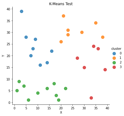
# cluster속성을 기준으로, df1데이터의 x와 y에 대해 그래프를 그리겠다.
# 즉, 그래프의 색상은 'cluster'를 기준으로 다르게 표현하겠다
sns.lmplot('x', 'y', data= df1, fit_reg= False, scatter_kws={'s':100},hue="cluster")
plt.title('K-Means Test')
plt.xlabel('X')
plt.ylabel('Y')
C:\Users\yein4\Anaconda3\lib\site-packages\seaborn\_decorators.py:43: FutureWarning: Pass the following variables as keyword args: x, y. From version 0.12, the only valid positional argument will be `data`, and passing other arguments without an explicit keyword will result in an error or misinterpretation.
  FutureWarning


Text(10.395989583333332, 0.5, 'Y')
K-Means | 실습2
import pandas as pd
import numpy as np
import seaborn as sns
from sklearn.cluster import KMeans # KMeans 리이브러리를 불러온다
from sklearn.datasets import load_iris # scikit-learn이 제공하는 샘플데이터 iris를 불러온다.
import matplotlib.pyplot as plt # 데이터 시각화를 위한 matplotlib을 불러온다
%matplotlib inline
K-Means | 실습2 | 데이터 확인
iris = load_iris()
# print(iris) # 뽑아보면 key와 value로 이루어진 것을 알 수 있다.
# Description 속성으로 데이터셋 정보를 확인한다.
# print(iris.DESCR)
print(iris)
{'data': array([[5.1, 3.5, 1.4, 0.2],
       [4.9, 3. , 1.4, 0.2],
       [4.7, 3.2, 1.3, 0.2],
       [4.6, 3.1, 1.5, 0.2],
       [5. , 3.6, 1.4, 0.2],
       [5.4, 3.9, 1.7, 0.4],
       [4.6, 3.4, 1.4, 0.3],
       [5. , 3.4, 1.5, 0.2],
       [4.4, 2.9, 1.4, 0.2],
       [4.9, 3.1, 1.5, 0.1],
       [5.4, 3.7, 1.5, 0.2],
       [4.8, 3.4, 1.6, 0.2],
       [4.8, 3. , 1.4, 0.1],
       [4.3, 3. , 1.1, 0.1],
       [5.8, 4. , 1.2, 0.2],
       [5.7, 4.4, 1.5, 0.4],
       [5.4, 3.9, 1.3, 0.4],
       [5.1, 3.5, 1.4, 0.3],
       [5.7, 3.8, 1.7, 0.3],
       [5.1, 3.8, 1.5, 0.3],
       [5.4, 3.4, 1.7, 0.2],
       [5.1, 3.7, 1.5, 0.4],
       [4.6, 3.6, 1. , 0.2],
       [5.1, 3.3, 1.7, 0.5],
       [4.8, 3.4, 1.9, 0.2],
       [5. , 3. , 1.6, 0.2],
       [5. , 3.4, 1.6, 0.4],
       [5.2, 3.5, 1.5, 0.2],
       [5.2, 3.4, 1.4, 0.2],
       [4.7, 3.2, 1.6, 0.2],
       [4.8, 3.1, 1.6, 0.2],
       [5.4, 3.4, 1.5, 0.4],
       [5.2, 4.1, 1.5, 0.1],
       [5.5, 4.2, 1.4, 0.2],
       [4.9, 3.1, 1.5, 0.2],
       [5. , 3.2, 1.2, 0.2],
       [5.5, 3.5, 1.3, 0.2],
       [4.9, 3.6, 1.4, 0.1],
       [4.4, 3. , 1.3, 0.2],
       [5.1, 3.4, 1.5, 0.2],
       [5. , 3.5, 1.3, 0.3],
       [4.5, 2.3, 1.3, 0.3],
       [4.4, 3.2, 1.3, 0.2],
       [5. , 3.5, 1.6, 0.6],
       [5.1, 3.8, 1.9, 0.4],
       [4.8, 3. , 1.4, 0.3],
       [5.1, 3.8, 1.6, 0.2],
       [4.6, 3.2, 1.4, 0.2],
       [5.3, 3.7, 1.5, 0.2],
       [5. , 3.3, 1.4, 0.2],
       [7. , 3.2, 4.7, 1.4],
       [6.4, 3.2, 4.5, 1.5],
       [6.9, 3.1, 4.9, 1.5],
       [5.5, 2.3, 4. , 1.3],
       [6.5, 2.8, 4.6, 1.5],
       [5.7, 2.8, 4.5, 1.3],
       [6.3, 3.3, 4.7, 1.6],
       [4.9, 2.4, 3.3, 1. ],
       [6.6, 2.9, 4.6, 1.3],
       [5.2, 2.7, 3.9, 1.4],
       [5. , 2. , 3.5, 1. ],
       [5.9, 3. , 4.2, 1.5],
       [6. , 2.2, 4. , 1. ],
       [6.1, 2.9, 4.7, 1.4],
       [5.6, 2.9, 3.6, 1.3],
       [6.7, 3.1, 4.4, 1.4],
       [5.6, 3. , 4.5, 1.5],
       [5.8, 2.7, 4.1, 1. ],
       [6.2, 2.2, 4.5, 1.5],
       [5.6, 2.5, 3.9, 1.1],
       [5.9, 3.2, 4.8, 1.8],
       [6.1, 2.8, 4. , 1.3],
       [6.3, 2.5, 4.9, 1.5],
       [6.1, 2.8, 4.7, 1.2],
       [6.4, 2.9, 4.3, 1.3],
       [6.6, 3. , 4.4, 1.4],
       [6.8, 2.8, 4.8, 1.4],
       [6.7, 3. , 5. , 1.7],
       [6. , 2.9, 4.5, 1.5],
       [5.7, 2.6, 3.5, 1. ],
       [5.5, 2.4, 3.8, 1.1],
       [5.5, 2.4, 3.7, 1. ],
       [5.8, 2.7, 3.9, 1.2],
       [6. , 2.7, 5.1, 1.6],
       [5.4, 3. , 4.5, 1.5],
       [6. , 3.4, 4.5, 1.6],
       [6.7, 3.1, 4.7, 1.5],
       [6.3, 2.3, 4.4, 1.3],
       [5.6, 3. , 4.1, 1.3],
       [5.5, 2.5, 4. , 1.3],
       [5.5, 2.6, 4.4, 1.2],
       [6.1, 3. , 4.6, 1.4],
       [5.8, 2.6, 4. , 1.2],
       [5. , 2.3, 3.3, 1. ],
       [5.6, 2.7, 4.2, 1.3],
       [5.7, 3. , 4.2, 1.2],
       [5.7, 2.9, 4.2, 1.3],
       [6.2, 2.9, 4.3, 1.3],
       [5.1, 2.5, 3. , 1.1],
       [5.7, 2.8, 4.1, 1.3],
       [6.3, 3.3, 6. , 2.5],
       [5.8, 2.7, 5.1, 1.9],
       [7.1, 3. , 5.9, 2.1],
       [6.3, 2.9, 5.6, 1.8],
       [6.5, 3. , 5.8, 2.2],
       [7.6, 3. , 6.6, 2.1],
       [4.9, 2.5, 4.5, 1.7],
       [7.3, 2.9, 6.3, 1.8],
       [6.7, 2.5, 5.8, 1.8],
       [7.2, 3.6, 6.1, 2.5],
       [6.5, 3.2, 5.1, 2. ],
       [6.4, 2.7, 5.3, 1.9],
       [6.8, 3. , 5.5, 2.1],
       [5.7, 2.5, 5. , 2. ],
       [5.8, 2.8, 5.1, 2.4],
       [6.4, 3.2, 5.3, 2.3],
       [6.5, 3. , 5.5, 1.8],
       [7.7, 3.8, 6.7, 2.2],
       [7.7, 2.6, 6.9, 2.3],
       [6. , 2.2, 5. , 1.5],
       [6.9, 3.2, 5.7, 2.3],
       [5.6, 2.8, 4.9, 2. ],
       [7.7, 2.8, 6.7, 2. ],
       [6.3, 2.7, 4.9, 1.8],
       [6.7, 3.3, 5.7, 2.1],
       [7.2, 3.2, 6. , 1.8],
       [6.2, 2.8, 4.8, 1.8],
       [6.1, 3. , 4.9, 1.8],
       [6.4, 2.8, 5.6, 2.1],
       [7.2, 3. , 5.8, 1.6],
       [7.4, 2.8, 6.1, 1.9],
       [7.9, 3.8, 6.4, 2. ],
       [6.4, 2.8, 5.6, 2.2],
       [6.3, 2.8, 5.1, 1.5],
       [6.1, 2.6, 5.6, 1.4],
       [7.7, 3. , 6.1, 2.3],
       [6.3, 3.4, 5.6, 2.4],
       [6.4, 3.1, 5.5, 1.8],
       [6. , 3. , 4.8, 1.8],
       [6.9, 3.1, 5.4, 2.1],
       [6.7, 3.1, 5.6, 2.4],
       [6.9, 3.1, 5.1, 2.3],
       [5.8, 2.7, 5.1, 1.9],
       [6.8, 3.2, 5.9, 2.3],
       [6.7, 3.3, 5.7, 2.5],
       [6.7, 3. , 5.2, 2.3],
       [6.3, 2.5, 5. , 1.9],
       [6.5, 3. , 5.2, 2. ],
       [6.2, 3.4, 5.4, 2.3],
       [5.9, 3. , 5.1, 1.8]]), 'target': array([0, 0, 0, 0, 0, 0, 0, 0, 0, 0, 0, 0, 0, 0, 0, 0, 0, 0, 0, 0, 0, 0,
       0, 0, 0, 0, 0, 0, 0, 0, 0, 0, 0, 0, 0, 0, 0, 0, 0, 0, 0, 0, 0, 0,
       0, 0, 0, 0, 0, 0, 1, 1, 1, 1, 1, 1, 1, 1, 1, 1, 1, 1, 1, 1, 1, 1,
       1, 1, 1, 1, 1, 1, 1, 1, 1, 1, 1, 1, 1, 1, 1, 1, 1, 1, 1, 1, 1, 1,
       1, 1, 1, 1, 1, 1, 1, 1, 1, 1, 1, 1, 2, 2, 2, 2, 2, 2, 2, 2, 2, 2,
       2, 2, 2, 2, 2, 2, 2, 2, 2, 2, 2, 2, 2, 2, 2, 2, 2, 2, 2, 2, 2, 2,
       2, 2, 2, 2, 2, 2, 2, 2, 2, 2, 2, 2, 2, 2, 2, 2, 2, 2]), 'frame': None, 'target_names': array(['setosa', 'versicolor', 'virginica'], dtype='<U10'), 'DESCR': '.. _iris_dataset:\n\nIris plants dataset\n--------------------\n\n**Data Set Characteristics:**\n\n    :Number of Instances: 150 (50 in each of three classes)\n    :Number of Attributes: 4 numeric, predictive attributes and the class\n    :Attribute Information:\n        - sepal length in cm\n        - sepal width in cm\n        - petal length in cm\n        - petal width in cm\n        - class:\n                - Iris-Setosa\n                - Iris-Versicolour\n                - Iris-Virginica\n                \n    :Summary Statistics:\n\n    ============== ==== ==== ======= ===== ====================\n                    Min  Max   Mean    SD   Class Correlation\n    ============== ==== ==== ======= ===== ====================\n    sepal length:   4.3  7.9   5.84   0.83    0.7826\n    sepal width:    2.0  4.4   3.05   0.43   -0.4194\n    petal length:   1.0  6.9   3.76   1.76    0.9490  (high!)\n    petal width:    0.1  2.5   1.20   0.76    0.9565  (high!)\n    ============== ==== ==== ======= ===== ====================\n\n    :Missing Attribute Values: None\n    :Class Distribution: 33.3% for each of 3 classes.\n    :Creator: R.A. Fisher\n    :Donor: Michael Marshall (MARSHALL%PLU@io.arc.nasa.gov)\n    :Date: July, 1988\n\nThe famous Iris database, first used by Sir R.A. Fisher. The dataset is taken\nfrom Fisher\'s paper. Note that it\'s the same as in R, but not as in the UCI\nMachine Learning Repository, which has two wrong data points.\n\nThis is perhaps the best known database to be found in the\npattern recognition literature.  Fisher\'s paper is a classic in the field and\nis referenced frequently to this day.  (See Duda & Hart, for example.)  The\ndata set contains 3 classes of 50 instances each, where each class refers to a\ntype of iris plant.  One class is linearly separable from the other 2; the\nlatter are NOT linearly separable from each other.\n\n.. topic:: References\n\n   - Fisher, R.A. "The use of multiple measurements in taxonomic problems"\n     Annual Eugenics, 7, Part II, 179-188 (1936); also in "Contributions to\n     Mathematical Statistics" (John Wiley, NY, 1950).\n   - Duda, R.O., & Hart, P.E. (1973) Pattern Classification and Scene Analysis.\n     (Q327.D83) John Wiley & Sons.  ISBN 0-471-22361-1.  See page 218.\n   - Dasarathy, B.V. (1980) "Nosing Around the Neighborhood: A New System\n     Structure and Classification Rule for Recognition in Partially Exposed\n     Environments".  IEEE Transactions on Pattern Analysis and Machine\n     Intelligence, Vol. PAMI-2, No. 1, 67-71.\n   - Gates, G.W. (1972) "The Reduced Nearest Neighbor Rule".  IEEE Transactions\n     on Information Theory, May 1972, 431-433.\n   - See also: 1988 MLC Proceedings, 54-64.  Cheeseman et al"s AUTOCLASS II\n     conceptual clustering system finds 3 classes in the data.\n   - Many, many more ...', 'feature_names': ['sepal length (cm)', 'sepal width (cm)', 'petal length (cm)', 'petal width (cm)'], 'filename': 'C:\\Users\\yein4\\Anaconda3\\lib\\site-packages\\sklearn\\datasets\\data\\iris.csv'}
print("key: ", iris.keys()) # key값을 뽑아본다.
key: dict_keys(['data', 'target', 'frame', 'target_names', 'DESCR', 'feature_names', 'filename'])
# data라는 key에 저장된 value의 인덱스 0부터 1까지 뽑아본다.
print("data: ", iris.data[0:3])
# feature_names라는 key에 저장된 value를 뽑아본다
print("feature_names: ", iris.feature_names)
data:  [[5.1 3.5 1.4 0.2]
 [4.9 3.  1.4 0.2]
 [4.7 3.2 1.3 0.2]]
feature_names:  ['sepal length (cm)', 'sepal width (cm)', 'petal length (cm)', 'petal width (cm)']
K-Means | 실습2 | 데이터 시각화
'''
아 그 전에 데이터가 어떻게 생겼는지 시각화하여 확인 먼저 해보자.
iris 데이터는 sepal length, sepal width, petal length, petal width
이렇게 총 4가지 feature를 가지고 있기 때문에 2차원 평만 상에 표현하기 위해서는
feature의 차원을 2개로 축소시켜 줘야 한다.
즉, 150 rows x 4 column -> 150 x 2로 만들어 줘야 한다.
4개의 feature를 2개로 축소하기 위해 PCA(Principal Component Analysis)를 사용하겠다.
'''
from sklearn.decomposition import PCA

# PCA를 위한 데이터프레임을 다시 만들어보자
iris_PCA_DF = pd.DataFrame(data = iris.data, columns = iris.feature_names)

# 출력 dimension을 설정한다. 여기에서는 2차원으로 출력을 원하니까 2.
pca = PCA(n_components = 2)
# PCA의 fit_transform 속성을 이용해 축소할 데이터를 넣는다.
pca_transformed = pca.fit_transform(iris.data)

# pca_transformed의 인덱스 0과 1을 각각 pca_x, pca_y라는 이름으로 데이터프레임에 추가해준다.
iris_PCA_DF['pca_x'] = pca_transformed[:,0]
iris_PCA_DF['pca_y'] = pca_transformed[:,1]
# iris의 종류를 나타내는 target을 데이터프레임에 추가해준다.
iris_PCA_DF['target'] = iris.target

# iris.target은 iris의 종류를 0, 1, 2로 표현한 데이터이다.
# iris.target_names로 iris 이름을 확인할 수 있다.
# 이름을 종류와 매핑해준다.
mappingDF = {0: 'Setosa', 1: 'Versicolour', 2: 'Virginica'}
# 데이터 프레임의 'target'값이 x에 들어가서 x가 0이면 mappingDF의 키값 0의 value값이 매핑된다.
iris_PCA_DF['target'] = iris_PCA_DF['target'].map(lambda x : mappingDF[x])

iris_PCA_DF.sample(5)
sepal length (cm)
sepal width (cm)
petal length (cm)
petal width (cm)
pca_x
pca_y
target
145
6.7
3.0
5.2
2.3
1.944110
0.187532
Virginica
40
5.0
3.5
1.3
0.3
-2.770102
0.263528
Setosa
13
4.3
3.0
1.1
0.1
-3.223804
-0.511395
Setosa
44
5.1
3.8
1.9
0.4
-2.209489
0.436663
Setosa
107
7.3
2.9
6.3
1.8
2.932587
0.355500
Virginica
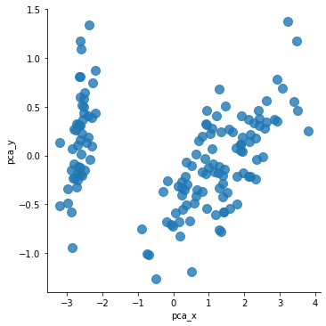
# target을 고려하지 않았을 때 데이터의 분포는 아래와 같다:
sns.lmplot('pca_x','pca_y', data= iris_PCA_DF, fit_reg=False, scatter_kws={'s': 100})
C:\Users\yein4\Anaconda3\lib\site-packages\seaborn\_decorators.py:43: FutureWarning: Pass the following variables as keyword args: x, y. From version 0.12, the only valid positional argument will be `data`, and passing other arguments without an explicit keyword will result in an error or misinterpretation.
  FutureWarning


<seaborn.axisgrid.FacetGrid at 0x12fbe7bff48>
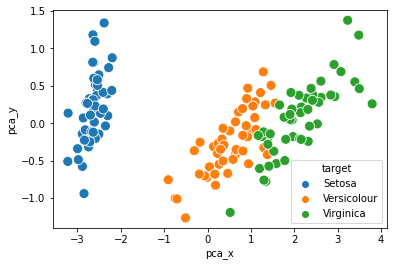
# target값을 고려해서 각 데이터의 이름이 반영되면 아래와 같아진다:
sns.scatterplot(x= 'pca_x', y = 'pca_y', data= iris_PCA_DF, hue=iris_PCA_DF['target'], s = 100)
<AxesSubplot:xlabel='pca_x', ylabel='pca_y'>
K-Means | 실습2 | K-Means 수행
# 이제 K-Means를 수행할 데이터프레임을 만들어보자
iris_KM_DF = pd.DataFrame(data = iris.data, columns = iris.feature_names)
print(iris_KM_DF.sample(5)) # 데이터프레임 5개만 뽑아서 확인해보자
     sepal length (cm)  sepal width (cm)  petal length (cm)  petal width (cm)
138                6.0               3.0                4.8               1.8
26                 5.0               3.4                1.6               0.4
47                 4.6               3.2                1.4               0.2
23                 5.1               3.3                1.7               0.5
112                6.8               3.0                5.5               2.1
# KMeans 라이브러리의 파라미터로 군집 개수, 최대 반복 횟수를 정해준다.
# iris데이터에서 종류는 3개니까 군집은 3개로, 최대 500번 돌고
# iris_DF라는 데이터프레임에 대해서 군집화를 시킨다.
kmeans1 = KMeans(n_clusters = 3, max_iter = 500, random_state = None).fit(iris_KM_DF)
kmeans1.cluster_centers_ # 각 클러스터들의 중심 위치를 뽑아본다.
array([[5.006     , 3.428     , 1.462     , 0.246     ],
       [5.9016129 , 2.7483871 , 4.39354839, 1.43387097],
       [6.85      , 3.07368421, 5.74210526, 2.07105263]])
# kmeans를 수행했으니까 각 데이터들이 속한 클러스터를 확인해보자
# 각 데이터의 인덱스에 해당 데이터의 소속 클러스터가 결과로 나온다.
kmeans1.labels_
array([0, 0, 0, 0, 0, 0, 0, 0, 0, 0, 0, 0, 0, 0, 0, 0, 0, 0, 0, 0, 0, 0,
       0, 0, 0, 0, 0, 0, 0, 0, 0, 0, 0, 0, 0, 0, 0, 0, 0, 0, 0, 0, 0, 0,
       0, 0, 0, 0, 0, 0, 1, 1, 2, 1, 1, 1, 1, 1, 1, 1, 1, 1, 1, 1, 1, 1,
       1, 1, 1, 1, 1, 1, 1, 1, 1, 1, 1, 2, 1, 1, 1, 1, 1, 1, 1, 1, 1, 1,
       1, 1, 1, 1, 1, 1, 1, 1, 1, 1, 1, 1, 2, 1, 2, 2, 2, 2, 1, 2, 2, 2,
       2, 2, 2, 1, 1, 2, 2, 2, 2, 1, 2, 1, 2, 1, 2, 2, 1, 1, 2, 2, 2, 2,
       2, 1, 2, 2, 2, 2, 1, 2, 2, 2, 1, 2, 2, 2, 1, 2, 2, 1])
# 데이터 프레임에 cluster라는 이름으로 각 데이터의 클러스터 결과를 넣어준다.
iris_KM_DF['cluster'] = kmeans1.labels_
# 데이터 프레임 인덱스 0부터 150까지 15씩 스탭한 결과를 출력해본다.
# (head를 뽑으면 앞쪽이 다 0이라 중간중간 결과들을 확인하기 위해)
iris_KM_DF[0:150:15]
# 총 3개의 클러스터가 존재하는 것을 확인할 수 있다.
sepal length (cm)
sepal width (cm)
petal length (cm)
petal width (cm)
cluster
0
5.1
3.5
1.4
0.2
0
15
5.7
4.4
1.5
0.4
0
30
4.8
3.1
1.6
0.2
0
45
4.8
3.0
1.4
0.3
0
60
5.0
2.0
3.5
1.0
1
75
6.6
3.0
4.4
1.4
1
90
5.5
2.6
4.4
1.2
1
105
7.6
3.0
6.6
2.1
2
120
6.9
3.2
5.7
2.3
2
135
7.7
3.0
6.1
2.3
2
# target값은 정답값이다.
# 클러스터링 결과를 대충 비교해보기 위해 데이터프레임에 넣어본다.
iris_KM_DF['target'] = iris.target
iris_KM_DF[10:150:15]
sepal length (cm)
sepal width (cm)
petal length (cm)
petal width (cm)
cluster
target
10
5.4
3.7
1.5
0.2
0
0
25
5.0
3.0
1.6
0.2
0
0
40
5.0
3.5
1.3
0.3
0
0
55
5.7
2.8
4.5
1.3
1
1
70
5.9
3.2
4.8
1.8
1
1
85
6.0
3.4
4.5
1.6
1
1
100
6.3
3.3
6.0
2.5
2
2
115
6.4
3.2
5.3
2.3
2
2
130
7.4
2.8
6.1
1.9
2
2
145
6.7
3.0
5.2
2.3
2
2
mappingDF = {0: 'Setosa', 1: 'Versicolour', 2: 'Virginica'}
# 데이터 프레임의 'target'값이 x에 들어가서 x가 0이면 mappingDF의 키값 0의 value값이 매핑된다.
iris_KM_DF['target'] = iris_KM_DF['target'].map(lambda x : mappingDF[x])
iris_KM_DF[10:150:15]
# 대충 봐도 클러스터링 결과와 정답값이 잘 맞는 것 같다.
sepal length (cm)
sepal width (cm)
petal length (cm)
petal width (cm)
cluster
target
10
5.4
3.7
1.5
0.2
0
Setosa
25
5.0
3.0
1.6
0.2
0
Setosa
40
5.0
3.5
1.3
0.3
0
Setosa
55
5.7
2.8
4.5
1.3
1
Versicolour
70
5.9
3.2
4.8
1.8
1
Versicolour
85
6.0
3.4
4.5
1.6
1
Versicolour
100
6.3
3.3
6.0
2.5
2
Virginica
115
6.4
3.2
5.3
2.3
2
Virginica
130
7.4
2.8
6.1
1.9
2
Virginica
145
6.7
3.0
5.2
2.3
2
Virginica
# 각 target에 대해 어떤 클러스터 결과가 존재하는지, 클러스터링 결과는 몇개인지 확인해보자
iris_result = iris_KM_DF.groupby(['target','cluster'])['sepal length (cm)'].count()
print(iris_result)
# 몇개는 군집화가 잘못 됐지만 거의 잘 된 것으로 확인된다.
target       cluster
Setosa       0          50
Versicolour  1          48
             2           2
Virginica    1          14
             2          36
Name: sepal length (cm), dtype: int64
# 위 과정을 함수로 만들어서 한번에 실행해보자
def KMEANS():
    iris = load_iris()

    iris_KM_DF2 = pd.DataFrame(data = iris.data, columns = iris.feature_names)

    kmeans = KMeans(n_clusters = 3, max_iter = 300, random_state = None).fit(iris_KM_DF2)
    kmeans.cluster_centers_

    iris_KM_DF2['cluster'] = kmeans.labels_
    iris_KM_DF2['target'] = iris.target

    mappingDF = {0: 'Setosa', 1: 'Versicolour', 2: 'Virginica'}
    iris_KM_DF2['target'] = iris_KM_DF2['target'].map(lambda x : mappingDF[x])

    iris_result = iris_KM_DF2.groupby(['target','cluster'])['sepal length (cm)'].count()
    print(iris_result)

KMEANS()
target       cluster
Setosa       0          50
Versicolour  1          48
             2           2
Virginica    1          14
             2          36
Name: sepal length (cm), dtype: int64
K-Means | 실습2 | K-Means 수행 결과 시각화
iris = load_iris()
iris_KM_VIS_DF = pd.DataFrame(data = iris.data, columns = iris.feature_names)
from sklearn.decomposition import PCA
def Visualize():
# 출력 dimension을 설정한다. 여기에서는 2차원으로 출력을 원하니까 2.
pca = PCA(n_components = 2)
# iris.data를 PCA로 변환시켜준다.
pca_transformed = pca.fit_transform(iris.data)
# PCA의 fit_transform 속성을 이용해 축소할 데이터를 넣는다.
iris_KM_VIS_DF['pca_x'] = pca_transformed[:,0]
iris_KM_VIS_DF['pca_y'] = pca_transformed[:,1]
# iris_KM_VIS_DF데이터프레임의 'cluster'의 값이 0, 1, 2 인 경우, 각각의 인덱스를 추출한다.
# cluster의 값이 0일 때 그 인덱스에 idx_0을 할당한다.
idx_0 = iris_KM_VIS_DF[iris_KM_VIS_DF['cluster'] == 0].index
idx_1 = iris_KM_VIS_DF[iris_KM_VIS_DF['cluster'] == 1].index
idx_2 = iris_KM_VIS_DF[iris_KM_VIS_DF['cluster'] == 2].index
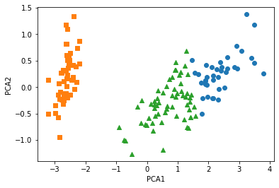
# 이제 그래프 그린다
fig, ax = plt.subplots()
# 각 군집 인덱스의 pca_x, pca_y 값 추출 및 시각화를 진행
# idx_0(cluster값이 0인 데이터의 인덱스)의 pca_x가 x,
# idx_0(cluster값이 0인 데이터의 인덱스)의 pca_y가 y인 지점은 동그라미로 표시
ax.scatter(x=iris_KM_VIS_DF.loc[idx_0, 'pca_x'], y= iris_KM_VIS_DF.loc[idx_0, 'pca_y'], marker = 'o')
ax.scatter(x=iris_KM_VIS_DF.loc[idx_1, 'pca_x'], y= iris_KM_VIS_DF.loc[idx_1, 'pca_y'], marker = 's')
ax.scatter(x=iris_KM_VIS_DF.loc[idx_2, 'pca_x'], y= iris_KM_VIS_DF.loc[idx_2, 'pca_y'], marker = '^')
ax.set_xlabel('PCA1')
ax.set_ylabel('PCA2')
def KMEANS_VIS():
    kmeans = KMeans(n_clusters = 3, max_iter = 300, random_state = None).fit(iris_KM_VIS_DF)
    kmeans.cluster_centers_

    iris_KM_VIS_DF['cluster'] = kmeans.labels_
    iris_KM_VIS_DF['target'] = iris.target

    mappingDF = {0: 'Setosa', 1: 'Versicolour', 2: 'Virginica'}
    iris_KM_VIS_DF['target'] = iris_KM_VIS_DF['target'].map(lambda x : mappingDF[x])

    #iris_result = iris_KM_VIS_DF.groupby(['target','cluster'])['sepal length (cm)'].count()
    #print(iris_result)
    Visualize()

print("K-Means 수행 결과:")
KMEANS_VIS()
K-Means 수행 결과:
# 정답값이랑 비교해보자
sns.scatterplot(x= 'pca_x', y = 'pca_y', data= iris_PCA_DF, hue=iris_PCA_DF['target'], s = 100)
<AxesSubplot:xlabel='pca_x', ylabel='pca_y'>

K-Means 실습 코드1: https://github.com/finddme/Finddme_Blog_Code/blob/master/Machine%20Learning/KMeans%EC%8B%A4%EC%8A%B51.ipynb
K-Means 실습 코드2: https://github.com/finddme/Finddme_Blog_Code/blob/master/Machine%20Learning/KMeans%EC%8B%A4%EC%8A%B52.ipynb
K-Means
-
K-Means는 클러스터링 알고리즘 중 하나이다. 클러스터링이란, 다량의 데이터를 군집화하는 기술로, 군집 간의 분산은 최대화하고 군집 내의 분산은 최소화하는 것이 목적인 알고리즘이다. K-Means알고리즘은 데이터의 영역을 대표하는 중심값(Cluster-center)을 찾아가며 데이터를 해당 Cluster에 할당하는 방식으로 작동한다.
-
데이터를 군집화하는 클러스터링과 같은 기술을은 대부분 비지도 학습 알고리즘이다. K-Means또한 비지도 학습 알고리즘에 속한다. 비지도 학습 알고리즘이란, 개발 시 정확한 작동 방향을 제시해주지 않아도 알아서 학습되는 알고리즘이다.(분류의 경우, 지도학습에 속한다)
-
K-means는 활용 분야가 매우 넓기 때문에 대표적인 데이터 마이닝 기술로 취급된다.
K-Means | 수행 과정
K-means는 EM알고리즘을 기반으로 작동된다. 즉, Expectation Step과 Maximization Step을 반복하며 학습한다. Expectation Step은 각 군집의 중심값을 찾는 단계이고, Maximization Step은 각 데이터들의 소속 클러스터를 갱신하는 단계이다. 두 단계를 수행한 후에는 중심값을 클러스터의 중앙으로 옮긴 후 다시 두 단계를 반복한다. 즉,
1. K-Means를 시작하면 중심값을 정하고, 중심에 가까운 데이터들을 해당 클러스터에 포함시킨다(EM알고리즘)
2. 중심값을 각 클러스터의 중앙으로 위치를 옮긴다.
위 두 과정을 반복하며 수행된다.
이러한 과정을 더이상 중심값의 위치가 변하지 않을 때까지 반복한다.
K-Means | 수행 준비
K-means를 수행하기 전,
1. 클러스터 개수
2. 클러스터링 수행 방식(무작위 중심값 선택, K-Means++ 등)
을 고려해 놔야 한다.
K-Means | 작동원리
위와 같은 데이터가 있을 때, 클러스터는 3개, K-Means++ 방식으로 클러스터링을 수행해보겠다.
1. 우선 맨 처음에 랜덤으로 특정한 원소 하나를 중심값으로 설정하고, 해당 값과 가장 먼 값을 골라준다.(K-Means++방식)
2. 그리고 두 중심값으로부터 가장 먼 원소를 또 다른 중심값으로 설정한다. 이렇게 중심값을 설정하면 세개의 중심값은 서로 가장 먼 위치에 자리하게 된다.
3. 각 데이터를 가장 가까운 중심값의 클러스터에 포함시킨다. 예를 들어 아래 그림의 회색 데이터는 1번 클러스터 중심값과 가장 가깝기 때문에 1번 클러스터에 소속된다.
모든 데이터들에 위와 같은 과정을 수행한다.
4. 군집화를 위와 같이 한 차례 마친 후에는 중심값들을 군집들의 중심으로 위치를 옮긴다.
그리고 다시 모든 데이터들이 각각 어느 클러스터의 중심값과 더 가까운지 확인해주고 기존에 소속된 클러스터의 중심값보다 다른 중심값이 더 가까우면 소속 클러스터를 변경해준다.
이러한 과정을 완전한 중심값을 찾을 때 까지, 즉 중심값이 더이상 변경되지 않을 때까지 반복한다.
K-Means | 실습1
from sklearn.cluster import KMeans # KMeans 라이브러리를 불러온다.
import numpy as np
import pandas as pd
import seaborn as sns # 데이터 시각화를 위한 seaborn과 matplotlib을 불러온다.
import matplotlib.pyplot as plt
%matplotlib inline
K-Means | 실습1 | 데이터 형성
# 데이터프레임을 하나 만든다.
df1 = pd.DataFrame(columns=['x','y'], dtype = 'float')
print(df1)
Empty DataFrame
Columns: [x, y]
Index: []
# 클러스터링을 수행할 데이터를 앞서 만든 데이터프레임에 채워준다.
# 좌표평면 위에 표현할 수 있는 데이터를 넣어준다. x축, y축.
# [x값, y값]
# 총 31개.
df1.loc[0] = [2, 9]
df1.loc[1] = [6, 1]
df1.loc[2] = [29, 30]
df1.loc[3] = [7, 20]
df1.loc[4] = [23, 31]
df1.loc[5] = [36, 23]
df1.loc[6] = [10, 4]
df1.loc[7] = [4, 7]
df1.loc[8] = [8, 23]
df1.loc[9] = [22, 6]
df1.loc[10] = [34, 24]
df1.loc[11] = [21, 37]
df1.loc[12] = [17, 8]
df1.loc[13] = [19, 1]
df1.loc[14] = [35, 34]
df1.loc[15] = [38, 28]
df1.loc[16] = [1, 5]
df1.loc[17] = [16, 22]
df1.loc[18] = [30, 15]
df1.loc[19] = [5, 28]
df1.loc[20] = [18, 3]
df1.loc[21] = [14, 17]
df1.loc[22] = [27, 19]
df1.loc[23] = [39, 14]
df1.loc[24] = [23, 29]
df1.loc[25] = [3, 39]
df1.loc[26] = [9, 27]
df1.loc[27] = [20, 26]
df1.loc[28] = [11, 16]
df1.loc[29] = [14, 6]
df1.loc[30] = [33, 2]
# head 함수를 사용해서 위에서 데이터를 하나하나 넣은 데이터프레임을 출력해본다.
df1.head(31)
| x | y | |
|---|---|---|
| 0 | 2.0 | 9.0 |
| 1 | 6.0 | 1.0 |
| 2 | 29.0 | 30.0 |
| 3 | 7.0 | 20.0 |
| 4 | 23.0 | 31.0 |
| 5 | 36.0 | 23.0 |
| 6 | 10.0 | 4.0 |
| 7 | 4.0 | 7.0 |
| 8 | 8.0 | 23.0 |
| 9 | 22.0 | 6.0 |
| 10 | 34.0 | 24.0 |
| 11 | 21.0 | 37.0 |
| 12 | 17.0 | 8.0 |
| 13 | 19.0 | 1.0 |
| 14 | 35.0 | 34.0 |
| 15 | 38.0 | 28.0 |
| 16 | 1.0 | 5.0 |
| 17 | 16.0 | 22.0 |
| 18 | 30.0 | 15.0 |
| 19 | 5.0 | 28.0 |
| 20 | 18.0 | 3.0 |
| 21 | 14.0 | 17.0 |
| 22 | 27.0 | 19.0 |
| 23 | 39.0 | 14.0 |
| 24 | 23.0 | 29.0 |
| 25 | 3.0 | 39.0 |
| 26 | 9.0 | 27.0 |
| 27 | 20.0 | 26.0 |
| 28 | 11.0 | 16.0 |
| 29 | 14.0 | 6.0 |
| 30 | 33.0 | 2.0 |
K-Means | 실습1 | 데이터 시각화
- 데이터 프레임을 만들어준 후에는 데이터를 그래프 형태로 보면 좋다. 데이터의 관계성 파악이 용이해진다.
'''
# 기호의 크기를 넣어줄 때는 scatter_kws매개변수에 대한 값을 딕셔너리 형태로 넣어주면 된다.
# seaborn라이브러리의 다변량 산점도 그래프를 그릴때 기호 크기 조절을 위해서
scatter_kws속성에 딕셔너리값의 key부분에 's'(size)를 넣어주면 된다.
# 그 다음 value부분에는 크기를 판별할 기준 변수를 넣어주면 된다
# fit_reg옵션으로 회귀선을 제거해줄 수 있다.
'''
# seaborn라이브러리에 있는 함수를 통해 df1데이터의 x와 y에 대해 그래프를 그리겠다고 한다.
sns.lmplot('x','y', data= df1, fit_reg=False, scatter_kws={'s': 100})
plt.title('DATA') # 위 그래프의 제목을 설정해줄 수 있다.
plt.xlabel('X') # x레이블은 X
plt.ylabel('Y') # y레이블은 Y
Text(10.049999999999997, 0.5, 'Y')
K-Means | 실습1 | K-Means 수행
# 이제 K-Means를 활용하여 클러스터링을 수행해보겠다.
points1 = df1.values # 연산 수행을 위해 데이터프레임의 값들을 numpy객체로서 초기화해준다.
points1[0:5]
array([[ 2., 9.],
[ 6., 1.],
[29., 30.],
[ 7., 20.],
[23., 31.]])
# 클러스터는 4개로 하고, ponits라는 데이터에 대해 K-Means를 수행한다.
# K-Means 클러스터링의 초기 군집 중심점 좌표 설정 방식은 K-Means++이 default이다.
kmeans1 = KMeans(n_clusters= 4).fit(points1)
kmeans1.cluster_centers_ # 각 클러스터들의 중심 위치를 뽑아본다.
# 4개의 클러스터 중심값의 위치(좌표)가 출력된다.
array([[ 9.125 , 24. ],
[27. , 30.71428571],
[11.3 , 5. ],
[33.16666667, 16.16666667]])
# kmeans를 수행했으니까 각 데이터들이 속한 클러스터를 확인해보자
# 각 데이터의 인덱스에 해당 데이터의 소속 클러스터가 결과로 나온다.
kmeans1.labels_
array([2, 2, 1, 0, 1, 3, 2, 2, 0, 2, 3, 1, 2, 2, 1, 1, 2, 0, 3, 0, 2, 0,
3, 3, 1, 0, 0, 1, 0, 2, 3])
# 시각화를 위해 'cluster'라는 이름으로 df1데이터프레임에 각 데이터의 클러스터 결과를 넣어준다.
df1['cluster'] = kmeans1.labels_
df1.head(5)
# 각 데이터들이 어떤 클러스터에 속하는지 출력된다.
| x | y | cluster | |
|---|---|---|---|
| 0 | 2.0 | 9.0 | 2 |
| 1 | 6.0 | 1.0 | 2 |
| 2 | 29.0 | 30.0 | 1 |
| 3 | 7.0 | 20.0 | 0 |
| 4 | 23.0 | 31.0 | 1 |
# cluster속성을 기준으로, df1데이터의 x와 y에 대해 그래프를 그리겠다.
# 즉, 그래프의 색상은 'cluster'를 기준으로 다르게 표현하겠다
sns.lmplot('x', 'y', data= df1, fit_reg= False, scatter_kws={'s':100},hue="cluster")
plt.title('K-Means Test')
plt.xlabel('X')
plt.ylabel('Y')
C:\Users\yein4\Anaconda3\lib\site-packages\seaborn\_decorators.py:43: FutureWarning: Pass the following variables as keyword args: x, y. From version 0.12, the only valid positional argument will be `data`, and passing other arguments without an explicit keyword will result in an error or misinterpretation.
FutureWarning
Text(10.395989583333332, 0.5, 'Y')
K-Means | 실습2
import pandas as pd
import numpy as np
import seaborn as sns
from sklearn.cluster import KMeans # KMeans 리이브러리를 불러온다
from sklearn.datasets import load_iris # scikit-learn이 제공하는 샘플데이터 iris를 불러온다.
import matplotlib.pyplot as plt # 데이터 시각화를 위한 matplotlib을 불러온다
%matplotlib inline
K-Means | 실습2 | 데이터 확인
iris = load_iris()
# print(iris) # 뽑아보면 key와 value로 이루어진 것을 알 수 있다.
# Description 속성으로 데이터셋 정보를 확인한다.
# print(iris.DESCR)
print(iris)
{'data': array([[5.1, 3.5, 1.4, 0.2],
[4.9, 3. , 1.4, 0.2],
[4.7, 3.2, 1.3, 0.2],
[4.6, 3.1, 1.5, 0.2],
[5. , 3.6, 1.4, 0.2],
[5.4, 3.9, 1.7, 0.4],
[4.6, 3.4, 1.4, 0.3],
[5. , 3.4, 1.5, 0.2],
[4.4, 2.9, 1.4, 0.2],
[4.9, 3.1, 1.5, 0.1],
[5.4, 3.7, 1.5, 0.2],
[4.8, 3.4, 1.6, 0.2],
[4.8, 3. , 1.4, 0.1],
[4.3, 3. , 1.1, 0.1],
[5.8, 4. , 1.2, 0.2],
[5.7, 4.4, 1.5, 0.4],
[5.4, 3.9, 1.3, 0.4],
[5.1, 3.5, 1.4, 0.3],
[5.7, 3.8, 1.7, 0.3],
[5.1, 3.8, 1.5, 0.3],
[5.4, 3.4, 1.7, 0.2],
[5.1, 3.7, 1.5, 0.4],
[4.6, 3.6, 1. , 0.2],
[5.1, 3.3, 1.7, 0.5],
[4.8, 3.4, 1.9, 0.2],
[5. , 3. , 1.6, 0.2],
[5. , 3.4, 1.6, 0.4],
[5.2, 3.5, 1.5, 0.2],
[5.2, 3.4, 1.4, 0.2],
[4.7, 3.2, 1.6, 0.2],
[4.8, 3.1, 1.6, 0.2],
[5.4, 3.4, 1.5, 0.4],
[5.2, 4.1, 1.5, 0.1],
[5.5, 4.2, 1.4, 0.2],
[4.9, 3.1, 1.5, 0.2],
[5. , 3.2, 1.2, 0.2],
[5.5, 3.5, 1.3, 0.2],
[4.9, 3.6, 1.4, 0.1],
[4.4, 3. , 1.3, 0.2],
[5.1, 3.4, 1.5, 0.2],
[5. , 3.5, 1.3, 0.3],
[4.5, 2.3, 1.3, 0.3],
[4.4, 3.2, 1.3, 0.2],
[5. , 3.5, 1.6, 0.6],
[5.1, 3.8, 1.9, 0.4],
[4.8, 3. , 1.4, 0.3],
[5.1, 3.8, 1.6, 0.2],
[4.6, 3.2, 1.4, 0.2],
[5.3, 3.7, 1.5, 0.2],
[5. , 3.3, 1.4, 0.2],
[7. , 3.2, 4.7, 1.4],
[6.4, 3.2, 4.5, 1.5],
[6.9, 3.1, 4.9, 1.5],
[5.5, 2.3, 4. , 1.3],
[6.5, 2.8, 4.6, 1.5],
[5.7, 2.8, 4.5, 1.3],
[6.3, 3.3, 4.7, 1.6],
[4.9, 2.4, 3.3, 1. ],
[6.6, 2.9, 4.6, 1.3],
[5.2, 2.7, 3.9, 1.4],
[5. , 2. , 3.5, 1. ],
[5.9, 3. , 4.2, 1.5],
[6. , 2.2, 4. , 1. ],
[6.1, 2.9, 4.7, 1.4],
[5.6, 2.9, 3.6, 1.3],
[6.7, 3.1, 4.4, 1.4],
[5.6, 3. , 4.5, 1.5],
[5.8, 2.7, 4.1, 1. ],
[6.2, 2.2, 4.5, 1.5],
[5.6, 2.5, 3.9, 1.1],
[5.9, 3.2, 4.8, 1.8],
[6.1, 2.8, 4. , 1.3],
[6.3, 2.5, 4.9, 1.5],
[6.1, 2.8, 4.7, 1.2],
[6.4, 2.9, 4.3, 1.3],
[6.6, 3. , 4.4, 1.4],
[6.8, 2.8, 4.8, 1.4],
[6.7, 3. , 5. , 1.7],
[6. , 2.9, 4.5, 1.5],
[5.7, 2.6, 3.5, 1. ],
[5.5, 2.4, 3.8, 1.1],
[5.5, 2.4, 3.7, 1. ],
[5.8, 2.7, 3.9, 1.2],
[6. , 2.7, 5.1, 1.6],
[5.4, 3. , 4.5, 1.5],
[6. , 3.4, 4.5, 1.6],
[6.7, 3.1, 4.7, 1.5],
[6.3, 2.3, 4.4, 1.3],
[5.6, 3. , 4.1, 1.3],
[5.5, 2.5, 4. , 1.3],
[5.5, 2.6, 4.4, 1.2],
[6.1, 3. , 4.6, 1.4],
[5.8, 2.6, 4. , 1.2],
[5. , 2.3, 3.3, 1. ],
[5.6, 2.7, 4.2, 1.3],
[5.7, 3. , 4.2, 1.2],
[5.7, 2.9, 4.2, 1.3],
[6.2, 2.9, 4.3, 1.3],
[5.1, 2.5, 3. , 1.1],
[5.7, 2.8, 4.1, 1.3],
[6.3, 3.3, 6. , 2.5],
[5.8, 2.7, 5.1, 1.9],
[7.1, 3. , 5.9, 2.1],
[6.3, 2.9, 5.6, 1.8],
[6.5, 3. , 5.8, 2.2],
[7.6, 3. , 6.6, 2.1],
[4.9, 2.5, 4.5, 1.7],
[7.3, 2.9, 6.3, 1.8],
[6.7, 2.5, 5.8, 1.8],
[7.2, 3.6, 6.1, 2.5],
[6.5, 3.2, 5.1, 2. ],
[6.4, 2.7, 5.3, 1.9],
[6.8, 3. , 5.5, 2.1],
[5.7, 2.5, 5. , 2. ],
[5.8, 2.8, 5.1, 2.4],
[6.4, 3.2, 5.3, 2.3],
[6.5, 3. , 5.5, 1.8],
[7.7, 3.8, 6.7, 2.2],
[7.7, 2.6, 6.9, 2.3],
[6. , 2.2, 5. , 1.5],
[6.9, 3.2, 5.7, 2.3],
[5.6, 2.8, 4.9, 2. ],
[7.7, 2.8, 6.7, 2. ],
[6.3, 2.7, 4.9, 1.8],
[6.7, 3.3, 5.7, 2.1],
[7.2, 3.2, 6. , 1.8],
[6.2, 2.8, 4.8, 1.8],
[6.1, 3. , 4.9, 1.8],
[6.4, 2.8, 5.6, 2.1],
[7.2, 3. , 5.8, 1.6],
[7.4, 2.8, 6.1, 1.9],
[7.9, 3.8, 6.4, 2. ],
[6.4, 2.8, 5.6, 2.2],
[6.3, 2.8, 5.1, 1.5],
[6.1, 2.6, 5.6, 1.4],
[7.7, 3. , 6.1, 2.3],
[6.3, 3.4, 5.6, 2.4],
[6.4, 3.1, 5.5, 1.8],
[6. , 3. , 4.8, 1.8],
[6.9, 3.1, 5.4, 2.1],
[6.7, 3.1, 5.6, 2.4],
[6.9, 3.1, 5.1, 2.3],
[5.8, 2.7, 5.1, 1.9],
[6.8, 3.2, 5.9, 2.3],
[6.7, 3.3, 5.7, 2.5],
[6.7, 3. , 5.2, 2.3],
[6.3, 2.5, 5. , 1.9],
[6.5, 3. , 5.2, 2. ],
[6.2, 3.4, 5.4, 2.3],
[5.9, 3. , 5.1, 1.8]]), 'target': array([0, 0, 0, 0, 0, 0, 0, 0, 0, 0, 0, 0, 0, 0, 0, 0, 0, 0, 0, 0, 0, 0,
0, 0, 0, 0, 0, 0, 0, 0, 0, 0, 0, 0, 0, 0, 0, 0, 0, 0, 0, 0, 0, 0,
0, 0, 0, 0, 0, 0, 1, 1, 1, 1, 1, 1, 1, 1, 1, 1, 1, 1, 1, 1, 1, 1,
1, 1, 1, 1, 1, 1, 1, 1, 1, 1, 1, 1, 1, 1, 1, 1, 1, 1, 1, 1, 1, 1,
1, 1, 1, 1, 1, 1, 1, 1, 1, 1, 1, 1, 2, 2, 2, 2, 2, 2, 2, 2, 2, 2,
2, 2, 2, 2, 2, 2, 2, 2, 2, 2, 2, 2, 2, 2, 2, 2, 2, 2, 2, 2, 2, 2,
2, 2, 2, 2, 2, 2, 2, 2, 2, 2, 2, 2, 2, 2, 2, 2, 2, 2]), 'frame': None, 'target_names': array(['setosa', 'versicolor', 'virginica'], dtype='<U10'), 'DESCR': '.. _iris_dataset:\n\nIris plants dataset\n--------------------\n\n**Data Set Characteristics:**\n\n :Number of Instances: 150 (50 in each of three classes)\n :Number of Attributes: 4 numeric, predictive attributes and the class\n :Attribute Information:\n - sepal length in cm\n - sepal width in cm\n - petal length in cm\n - petal width in cm\n - class:\n - Iris-Setosa\n - Iris-Versicolour\n - Iris-Virginica\n \n :Summary Statistics:\n\n ============== ==== ==== ======= ===== ====================\n Min Max Mean SD Class Correlation\n ============== ==== ==== ======= ===== ====================\n sepal length: 4.3 7.9 5.84 0.83 0.7826\n sepal width: 2.0 4.4 3.05 0.43 -0.4194\n petal length: 1.0 6.9 3.76 1.76 0.9490 (high!)\n petal width: 0.1 2.5 1.20 0.76 0.9565 (high!)\n ============== ==== ==== ======= ===== ====================\n\n :Missing Attribute Values: None\n :Class Distribution: 33.3% for each of 3 classes.\n :Creator: R.A. Fisher\n :Donor: Michael Marshall (MARSHALL%PLU@io.arc.nasa.gov)\n :Date: July, 1988\n\nThe famous Iris database, first used by Sir R.A. Fisher. The dataset is taken\nfrom Fisher\'s paper. Note that it\'s the same as in R, but not as in the UCI\nMachine Learning Repository, which has two wrong data points.\n\nThis is perhaps the best known database to be found in the\npattern recognition literature. Fisher\'s paper is a classic in the field and\nis referenced frequently to this day. (See Duda & Hart, for example.) The\ndata set contains 3 classes of 50 instances each, where each class refers to a\ntype of iris plant. One class is linearly separable from the other 2; the\nlatter are NOT linearly separable from each other.\n\n.. topic:: References\n\n - Fisher, R.A. "The use of multiple measurements in taxonomic problems"\n Annual Eugenics, 7, Part II, 179-188 (1936); also in "Contributions to\n Mathematical Statistics" (John Wiley, NY, 1950).\n - Duda, R.O., & Hart, P.E. (1973) Pattern Classification and Scene Analysis.\n (Q327.D83) John Wiley & Sons. ISBN 0-471-22361-1. See page 218.\n - Dasarathy, B.V. (1980) "Nosing Around the Neighborhood: A New System\n Structure and Classification Rule for Recognition in Partially Exposed\n Environments". IEEE Transactions on Pattern Analysis and Machine\n Intelligence, Vol. PAMI-2, No. 1, 67-71.\n - Gates, G.W. (1972) "The Reduced Nearest Neighbor Rule". IEEE Transactions\n on Information Theory, May 1972, 431-433.\n - See also: 1988 MLC Proceedings, 54-64. Cheeseman et al"s AUTOCLASS II\n conceptual clustering system finds 3 classes in the data.\n - Many, many more ...', 'feature_names': ['sepal length (cm)', 'sepal width (cm)', 'petal length (cm)', 'petal width (cm)'], 'filename': 'C:\\Users\\yein4\\Anaconda3\\lib\\site-packages\\sklearn\\datasets\\data\\iris.csv'}
print("key: ", iris.keys()) # key값을 뽑아본다.
key: dict_keys(['data', 'target', 'frame', 'target_names', 'DESCR', 'feature_names', 'filename'])
# data라는 key에 저장된 value의 인덱스 0부터 1까지 뽑아본다.
print("data: ", iris.data[0:3])
# feature_names라는 key에 저장된 value를 뽑아본다
print("feature_names: ", iris.feature_names)
data: [[5.1 3.5 1.4 0.2]
[4.9 3. 1.4 0.2]
[4.7 3.2 1.3 0.2]]
feature_names: ['sepal length (cm)', 'sepal width (cm)', 'petal length (cm)', 'petal width (cm)']
K-Means | 실습2 | 데이터 시각화
'''
아 그 전에 데이터가 어떻게 생겼는지 시각화하여 확인 먼저 해보자.
iris 데이터는 sepal length, sepal width, petal length, petal width
이렇게 총 4가지 feature를 가지고 있기 때문에 2차원 평만 상에 표현하기 위해서는
feature의 차원을 2개로 축소시켜 줘야 한다.
즉, 150 rows x 4 column -> 150 x 2로 만들어 줘야 한다.
4개의 feature를 2개로 축소하기 위해 PCA(Principal Component Analysis)를 사용하겠다.
'''
from sklearn.decomposition import PCA
# PCA를 위한 데이터프레임을 다시 만들어보자
iris_PCA_DF = pd.DataFrame(data = iris.data, columns = iris.feature_names)
# 출력 dimension을 설정한다. 여기에서는 2차원으로 출력을 원하니까 2.
pca = PCA(n_components = 2)
# PCA의 fit_transform 속성을 이용해 축소할 데이터를 넣는다.
pca_transformed = pca.fit_transform(iris.data)
# pca_transformed의 인덱스 0과 1을 각각 pca_x, pca_y라는 이름으로 데이터프레임에 추가해준다.
iris_PCA_DF['pca_x'] = pca_transformed[:,0]
iris_PCA_DF['pca_y'] = pca_transformed[:,1]
# iris의 종류를 나타내는 target을 데이터프레임에 추가해준다.
iris_PCA_DF['target'] = iris.target
# iris.target은 iris의 종류를 0, 1, 2로 표현한 데이터이다.
# iris.target_names로 iris 이름을 확인할 수 있다.
# 이름을 종류와 매핑해준다.
mappingDF = {0: 'Setosa', 1: 'Versicolour', 2: 'Virginica'}
# 데이터 프레임의 'target'값이 x에 들어가서 x가 0이면 mappingDF의 키값 0의 value값이 매핑된다.
iris_PCA_DF['target'] = iris_PCA_DF['target'].map(lambda x : mappingDF[x])
iris_PCA_DF.sample(5)
| sepal length (cm) | sepal width (cm) | petal length (cm) | petal width (cm) | pca_x | pca_y | target | |
|---|---|---|---|---|---|---|---|
| 145 | 6.7 | 3.0 | 5.2 | 2.3 | 1.944110 | 0.187532 | Virginica |
| 40 | 5.0 | 3.5 | 1.3 | 0.3 | -2.770102 | 0.263528 | Setosa |
| 13 | 4.3 | 3.0 | 1.1 | 0.1 | -3.223804 | -0.511395 | Setosa |
| 44 | 5.1 | 3.8 | 1.9 | 0.4 | -2.209489 | 0.436663 | Setosa |
| 107 | 7.3 | 2.9 | 6.3 | 1.8 | 2.932587 | 0.355500 | Virginica |
# target을 고려하지 않았을 때 데이터의 분포는 아래와 같다:
sns.lmplot('pca_x','pca_y', data= iris_PCA_DF, fit_reg=False, scatter_kws={'s': 100})
C:\Users\yein4\Anaconda3\lib\site-packages\seaborn\_decorators.py:43: FutureWarning: Pass the following variables as keyword args: x, y. From version 0.12, the only valid positional argument will be `data`, and passing other arguments without an explicit keyword will result in an error or misinterpretation.
FutureWarning
<seaborn.axisgrid.FacetGrid at 0x12fbe7bff48>
# target값을 고려해서 각 데이터의 이름이 반영되면 아래와 같아진다:
sns.scatterplot(x= 'pca_x', y = 'pca_y', data= iris_PCA_DF, hue=iris_PCA_DF['target'], s = 100)
<AxesSubplot:xlabel='pca_x', ylabel='pca_y'>
K-Means | 실습2 | K-Means 수행
# 이제 K-Means를 수행할 데이터프레임을 만들어보자
iris_KM_DF = pd.DataFrame(data = iris.data, columns = iris.feature_names)
print(iris_KM_DF.sample(5)) # 데이터프레임 5개만 뽑아서 확인해보자
sepal length (cm) sepal width (cm) petal length (cm) petal width (cm)
138 6.0 3.0 4.8 1.8
26 5.0 3.4 1.6 0.4
47 4.6 3.2 1.4 0.2
23 5.1 3.3 1.7 0.5
112 6.8 3.0 5.5 2.1
# KMeans 라이브러리의 파라미터로 군집 개수, 최대 반복 횟수를 정해준다.
# iris데이터에서 종류는 3개니까 군집은 3개로, 최대 500번 돌고
# iris_DF라는 데이터프레임에 대해서 군집화를 시킨다.
kmeans1 = KMeans(n_clusters = 3, max_iter = 500, random_state = None).fit(iris_KM_DF)
kmeans1.cluster_centers_ # 각 클러스터들의 중심 위치를 뽑아본다.
array([[5.006 , 3.428 , 1.462 , 0.246 ],
[5.9016129 , 2.7483871 , 4.39354839, 1.43387097],
[6.85 , 3.07368421, 5.74210526, 2.07105263]])
# kmeans를 수행했으니까 각 데이터들이 속한 클러스터를 확인해보자
# 각 데이터의 인덱스에 해당 데이터의 소속 클러스터가 결과로 나온다.
kmeans1.labels_
array([0, 0, 0, 0, 0, 0, 0, 0, 0, 0, 0, 0, 0, 0, 0, 0, 0, 0, 0, 0, 0, 0,
0, 0, 0, 0, 0, 0, 0, 0, 0, 0, 0, 0, 0, 0, 0, 0, 0, 0, 0, 0, 0, 0,
0, 0, 0, 0, 0, 0, 1, 1, 2, 1, 1, 1, 1, 1, 1, 1, 1, 1, 1, 1, 1, 1,
1, 1, 1, 1, 1, 1, 1, 1, 1, 1, 1, 2, 1, 1, 1, 1, 1, 1, 1, 1, 1, 1,
1, 1, 1, 1, 1, 1, 1, 1, 1, 1, 1, 1, 2, 1, 2, 2, 2, 2, 1, 2, 2, 2,
2, 2, 2, 1, 1, 2, 2, 2, 2, 1, 2, 1, 2, 1, 2, 2, 1, 1, 2, 2, 2, 2,
2, 1, 2, 2, 2, 2, 1, 2, 2, 2, 1, 2, 2, 2, 1, 2, 2, 1])
# 데이터 프레임에 cluster라는 이름으로 각 데이터의 클러스터 결과를 넣어준다.
iris_KM_DF['cluster'] = kmeans1.labels_
# 데이터 프레임 인덱스 0부터 150까지 15씩 스탭한 결과를 출력해본다.
# (head를 뽑으면 앞쪽이 다 0이라 중간중간 결과들을 확인하기 위해)
iris_KM_DF[0:150:15]
# 총 3개의 클러스터가 존재하는 것을 확인할 수 있다.
| sepal length (cm) | sepal width (cm) | petal length (cm) | petal width (cm) | cluster | |
|---|---|---|---|---|---|
| 0 | 5.1 | 3.5 | 1.4 | 0.2 | 0 |
| 15 | 5.7 | 4.4 | 1.5 | 0.4 | 0 |
| 30 | 4.8 | 3.1 | 1.6 | 0.2 | 0 |
| 45 | 4.8 | 3.0 | 1.4 | 0.3 | 0 |
| 60 | 5.0 | 2.0 | 3.5 | 1.0 | 1 |
| 75 | 6.6 | 3.0 | 4.4 | 1.4 | 1 |
| 90 | 5.5 | 2.6 | 4.4 | 1.2 | 1 |
| 105 | 7.6 | 3.0 | 6.6 | 2.1 | 2 |
| 120 | 6.9 | 3.2 | 5.7 | 2.3 | 2 |
| 135 | 7.7 | 3.0 | 6.1 | 2.3 | 2 |
# target값은 정답값이다.
# 클러스터링 결과를 대충 비교해보기 위해 데이터프레임에 넣어본다.
iris_KM_DF['target'] = iris.target
iris_KM_DF[10:150:15]
| sepal length (cm) | sepal width (cm) | petal length (cm) | petal width (cm) | cluster | target | |
|---|---|---|---|---|---|---|
| 10 | 5.4 | 3.7 | 1.5 | 0.2 | 0 | 0 |
| 25 | 5.0 | 3.0 | 1.6 | 0.2 | 0 | 0 |
| 40 | 5.0 | 3.5 | 1.3 | 0.3 | 0 | 0 |
| 55 | 5.7 | 2.8 | 4.5 | 1.3 | 1 | 1 |
| 70 | 5.9 | 3.2 | 4.8 | 1.8 | 1 | 1 |
| 85 | 6.0 | 3.4 | 4.5 | 1.6 | 1 | 1 |
| 100 | 6.3 | 3.3 | 6.0 | 2.5 | 2 | 2 |
| 115 | 6.4 | 3.2 | 5.3 | 2.3 | 2 | 2 |
| 130 | 7.4 | 2.8 | 6.1 | 1.9 | 2 | 2 |
| 145 | 6.7 | 3.0 | 5.2 | 2.3 | 2 | 2 |
mappingDF = {0: 'Setosa', 1: 'Versicolour', 2: 'Virginica'}
# 데이터 프레임의 'target'값이 x에 들어가서 x가 0이면 mappingDF의 키값 0의 value값이 매핑된다.
iris_KM_DF['target'] = iris_KM_DF['target'].map(lambda x : mappingDF[x])
iris_KM_DF[10:150:15]
# 대충 봐도 클러스터링 결과와 정답값이 잘 맞는 것 같다.
| sepal length (cm) | sepal width (cm) | petal length (cm) | petal width (cm) | cluster | target | |
|---|---|---|---|---|---|---|
| 10 | 5.4 | 3.7 | 1.5 | 0.2 | 0 | Setosa |
| 25 | 5.0 | 3.0 | 1.6 | 0.2 | 0 | Setosa |
| 40 | 5.0 | 3.5 | 1.3 | 0.3 | 0 | Setosa |
| 55 | 5.7 | 2.8 | 4.5 | 1.3 | 1 | Versicolour |
| 70 | 5.9 | 3.2 | 4.8 | 1.8 | 1 | Versicolour |
| 85 | 6.0 | 3.4 | 4.5 | 1.6 | 1 | Versicolour |
| 100 | 6.3 | 3.3 | 6.0 | 2.5 | 2 | Virginica |
| 115 | 6.4 | 3.2 | 5.3 | 2.3 | 2 | Virginica |
| 130 | 7.4 | 2.8 | 6.1 | 1.9 | 2 | Virginica |
| 145 | 6.7 | 3.0 | 5.2 | 2.3 | 2 | Virginica |
# 각 target에 대해 어떤 클러스터 결과가 존재하는지, 클러스터링 결과는 몇개인지 확인해보자
iris_result = iris_KM_DF.groupby(['target','cluster'])['sepal length (cm)'].count()
print(iris_result)
# 몇개는 군집화가 잘못 됐지만 거의 잘 된 것으로 확인된다.
target cluster
Setosa 0 50
Versicolour 1 48
2 2
Virginica 1 14
2 36
Name: sepal length (cm), dtype: int64
# 위 과정을 함수로 만들어서 한번에 실행해보자
def KMEANS():
iris = load_iris()
iris_KM_DF2 = pd.DataFrame(data = iris.data, columns = iris.feature_names)
kmeans = KMeans(n_clusters = 3, max_iter = 300, random_state = None).fit(iris_KM_DF2)
kmeans.cluster_centers_
iris_KM_DF2['cluster'] = kmeans.labels_
iris_KM_DF2['target'] = iris.target
mappingDF = {0: 'Setosa', 1: 'Versicolour', 2: 'Virginica'}
iris_KM_DF2['target'] = iris_KM_DF2['target'].map(lambda x : mappingDF[x])
iris_result = iris_KM_DF2.groupby(['target','cluster'])['sepal length (cm)'].count()
print(iris_result)
KMEANS()
target cluster
Setosa 0 50
Versicolour 1 48
2 2
Virginica 1 14
2 36
Name: sepal length (cm), dtype: int64
K-Means | 실습2 | K-Means 수행 결과 시각화
iris = load_iris()
iris_KM_VIS_DF = pd.DataFrame(data = iris.data, columns = iris.feature_names)
from sklearn.decomposition import PCA
def Visualize():
# 출력 dimension을 설정한다. 여기에서는 2차원으로 출력을 원하니까 2.
pca = PCA(n_components = 2)
# iris.data를 PCA로 변환시켜준다.
pca_transformed = pca.fit_transform(iris.data)
# PCA의 fit_transform 속성을 이용해 축소할 데이터를 넣는다.
iris_KM_VIS_DF['pca_x'] = pca_transformed[:,0]
iris_KM_VIS_DF['pca_y'] = pca_transformed[:,1]
# iris_KM_VIS_DF데이터프레임의 'cluster'의 값이 0, 1, 2 인 경우, 각각의 인덱스를 추출한다.
# cluster의 값이 0일 때 그 인덱스에 idx_0을 할당한다.
idx_0 = iris_KM_VIS_DF[iris_KM_VIS_DF['cluster'] == 0].index
idx_1 = iris_KM_VIS_DF[iris_KM_VIS_DF['cluster'] == 1].index
idx_2 = iris_KM_VIS_DF[iris_KM_VIS_DF['cluster'] == 2].index
# 이제 그래프 그린다
fig, ax = plt.subplots()
# 각 군집 인덱스의 pca_x, pca_y 값 추출 및 시각화를 진행
# idx_0(cluster값이 0인 데이터의 인덱스)의 pca_x가 x,
# idx_0(cluster값이 0인 데이터의 인덱스)의 pca_y가 y인 지점은 동그라미로 표시
ax.scatter(x=iris_KM_VIS_DF.loc[idx_0, 'pca_x'], y= iris_KM_VIS_DF.loc[idx_0, 'pca_y'], marker = 'o')
ax.scatter(x=iris_KM_VIS_DF.loc[idx_1, 'pca_x'], y= iris_KM_VIS_DF.loc[idx_1, 'pca_y'], marker = 's')
ax.scatter(x=iris_KM_VIS_DF.loc[idx_2, 'pca_x'], y= iris_KM_VIS_DF.loc[idx_2, 'pca_y'], marker = '^')
ax.set_xlabel('PCA1')
ax.set_ylabel('PCA2')
def KMEANS_VIS():
kmeans = KMeans(n_clusters = 3, max_iter = 300, random_state = None).fit(iris_KM_VIS_DF)
kmeans.cluster_centers_
iris_KM_VIS_DF['cluster'] = kmeans.labels_
iris_KM_VIS_DF['target'] = iris.target
mappingDF = {0: 'Setosa', 1: 'Versicolour', 2: 'Virginica'}
iris_KM_VIS_DF['target'] = iris_KM_VIS_DF['target'].map(lambda x : mappingDF[x])
#iris_result = iris_KM_VIS_DF.groupby(['target','cluster'])['sepal length (cm)'].count()
#print(iris_result)
Visualize()
print("K-Means 수행 결과:")
KMEANS_VIS()
K-Means 수행 결과:
# 정답값이랑 비교해보자
sns.scatterplot(x= 'pca_x', y = 'pca_y', data= iris_PCA_DF, hue=iris_PCA_DF['target'], s = 100)
<AxesSubplot:xlabel='pca_x', ylabel='pca_y'>